Top 20 MS Excel Formulas and Function: Learn with Example

Microsoft Excel is one of the world’s most popular spreadsheet software used for a variety of book-keeping and data storage purposes. But its use is not limited to just recording data, it is also a tool filled with potential for data analysis and calculations. To use the various computational features of MS Excel, there are a number of basic formulae and functions that you must be aware of. 

However, if you are not a tech-savvy person, here we have made the job easier for you by listing down the basic formulae in MS Excel along with step-by-step guides of how to run them and continue reading to explore. 

Basic Formulae and Functions of M.S Excel: Know the Difference

MS Excel has 2 main facilities for running mathematical operations on data. These include formulae and functions, which are closely related to each other but have one fundamental difference between each other: 

• A formula in Excel is a command for a mathematical operation that you feed into Excel. An example of a formula would be “=A4+C4” 
• A function is a predefined command for a mathematical operation in Excel which has a set syntax and format. A simple function in Excel is the SUM function used as “=SUM (A2:B2)” 

Notice that one needs to manually feed the info about the cells to be added in the case of a formula (you will need to feed the data about 5 cells manually if you wish to add those 5 cells) while in the case of a function, you can use the SUM function directly and just enter the values of the cell (e.g. A2 to E2 represented as A2:E2) for the software to automatically calculate the sum of the cell values. 

Functions are easier to use as compared to formulae in Excel since they come with pre-designed syntax and can directly be used to perform various operations with the data. 

Another major advantage of using a function in Excel is that there are many operations and commands for which it is not possible to directly feed a formula manually to the software. In such cases, there are many functions of Excel which can be used to directly run the command. 

Video Source: Kevin Stratvert

Formulae and Functions: Syntax of a Formula and Function 

Before proceeding onto using the actual formulae and functions in Excel, one needs to have a basic understanding of what is the structure of a formula or function, which is referred to as the “syntax”. 

For a formula, the syntax includes an equal sign (“=”) followed by the operation you wish to perform along with the relevant cell references. For example if you need to find the product between cells A1 and D5, we can create a formula as follows: 

• =A1*D5 

For a function for the same operation, we shall begin with the equal sign (“=”) followed by the function command we wish to perform (e.g. PRODUCT in our case), followed by a bracket wherein the cell references are provided in which the function is to be performed. So for the above example, the function to use is PRODUCT and the syntax will be: 

• =PRODUCT(A1,B2)

Here, since we are already providing the function PRODUCT outside the brackets, we do not enter an asterisk  (“*”) sign rather we separate the two cell values through a simple comma (“,”). 

For some functions, instead of the comma (,) one needs to use the colon (“:”) instead which denotes a series of cells rather than a couple of cells on which the operation is to be performed. 

Given below is an easy tutorial on how to use the various functions and formulae in MS Excel along with the use cases for those functions. 

Step-by-Step Guide for Top 20 MS Excel Formulae 

1) SUM Function

This is the simplest function of the software and it is used to calculate the additive sum of the cells you feed into the command. The function command begins with an equal sign (“=”) followed by the main command  (“SUM”), followed by the cells whose values are to be added. 

You can enter the cell command in terms of specific cells (separated by a comma) or a series of cells (separated by a colon- “:”). The command is: 

=SUM(starting cell:ending cell)

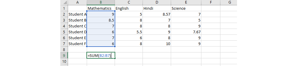
• Enter the command- =SUM(
• Now select the cells you wish to add, these will be visible within the brackets of your command
• Close the command with a bracket -“)” 
• Press Enter 
• The sum of the reference cell values will be displayed in the cell. 

2) SUMIF Function 

The SUMIF function is an extension of the SUM function, in which we add a condition about the sum, for example-only adding cell values when they exceed a particular value. This function is useful for screening particular values from a dataset and performing the addition only on specific cell values. 

The syntax of this command is similar to the SUM command, but includes an additional subcommand about the condition you want to place on the cell values. 

• It starts with an equal sign (=) followed by the main command- SUMIF
• This is followed by a bracket within which you enter the cell values (e.g. A2:F2)
• After entering the cell values, put a comma (“,”), followed by your condition (e.g >5) in double inverted commas. 
• The command closes with the bracket.
• So the final syntax of the command is-

=SUMIF(start cell: end cell, “Condition”)

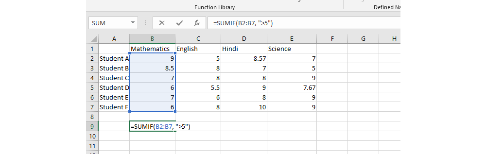
In the given dataset, if you want to find out the sum of scores for students who have scored more than 5 marks in the mathematics exam, then you can use the command

=SUMIF(B2:B7, “>5”). 

3) AVERAGE Function 

As understandable from the name of the command itself, the AVERAGE function is used to find the average or the arithmetic mean of the cells. This is a very useful function for data keeping and is one of the simplest to run in MS Excel. 

The syntax of the command is an equal sign (“=”), followed by the main command AVERAGE, followed by a bracket in which you provide the relevant reference cells of which you want to find the average, followed by a bracket to close the command. The final syntax is 

=AVERAGE(starting cell:end cell)

=AVERAGE(cell values separated by comma)

 
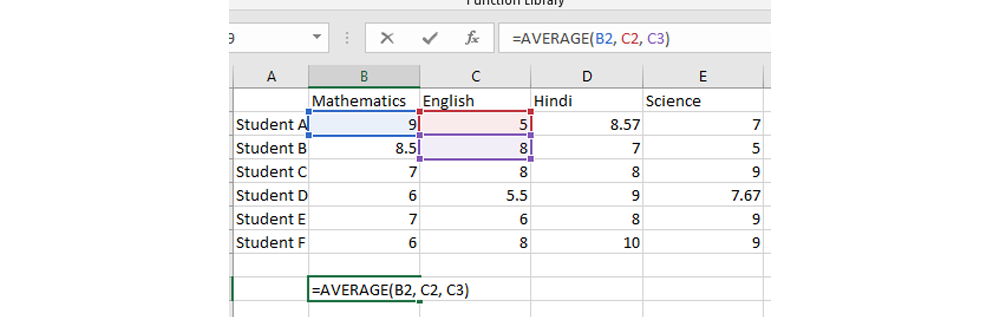
For example, here if you want to calculate the average of the cells B1,C2 and C3, the syntax will be 

• =AVERAGE(B1, C2, C3)

This feature is useful for calculating the average in a dataset for a variety of purposes. 

4) MEDIAN Function 

For some statistical procedures or computational tasks, one needs to find out the middle-most value in the set of values. This value is called the median in statistical terms, and can be calculated using the MEDIAN function in MS Excel. 

This command has a simple syntax in which we start with an equal sign (“=”), followed by the main command- MEDIAN, followed by the cells of which we must find the median, separated by a colon. The command is then closed with a bracket. So the syntax of the function is: 

=MEDIAN(starting cell value:ending cell value) 

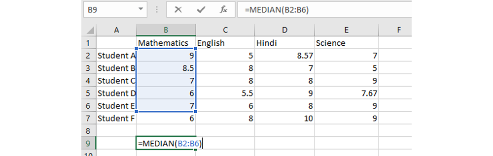
For example, in the given dataset, if you want to find the median value of the cells B2 to B6, simply enter the command =MEDIAN(B2:B6) and Excel will find the median value for you. 

5) COUNT Function 

Consider an example if you have a huge dataset in which you want to find the total number of values in a row of data. To calculate the number of entries in a dataset, you can use the COUNT function of Excel. 

The syntax of the command includes an equal sign (“=”), followed by the main command- COUNT, followed by a bracket which encloses the reference cell values. The command is then closed with a bracket, and upon pressing the Enter key, the number of values is calculated. So the final syntax of the COUNT function is

=COUNT(starting cell:ending cell)

This command does not calculate the cells which are blank or have data in any other form other than numerical data in the total count. 

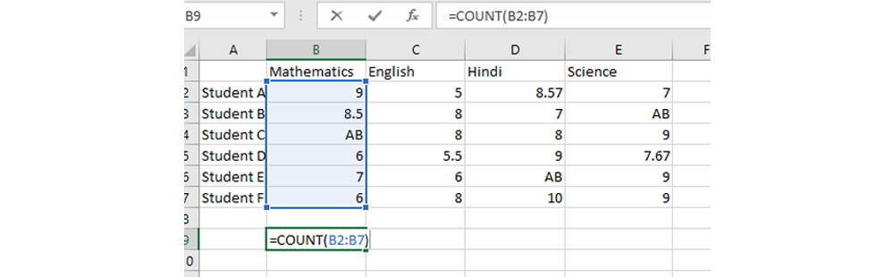
For example, in this case, if you want to calculate the total number of students who appeared for the test of mathematics, you can use the COUNT function as follows: 

=COUNT(B2:B7)

This command eliminates empty cells and textual cells in the calculation of the total count. 

6) COUNTA Function 

COUNTA function is an extended function related to the COUNT command, and it also includes  cells with textual or other data forms for calculating the total cells. This command is useful when you don’t want to omit cells with textual content from your total count. 

The syntax of the command is similar to the COUNT function, except the main command used is COUNTA instead of COUNT. So the syntax of the command is 

=COUNTA(starting cell: ending cell)

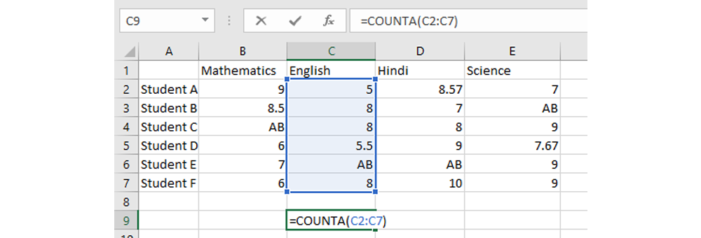
For example, if you want to calculate the total number of students in a class, including the absentees for a particular test, you can use the COUNTA function as follows: 

=COUNTA(C2:C7)

This command will give you the total count of cells from the C2 to C7 range of cells. 

7) SUBTOTAL Function 

The SUBTOTAL function is slightly different from the functions mentioned prior to it, in that it performs a function on a sublist in a dataset. It includes a subcommand within a main command, and these subcommands are represented in the syntax using certain numbers which denote various subcommands. 

The syntax of the command includes an equal sign (“=”) followed by the main command which is SUBTOTAL, followed by a bracket, within which you first provide the subcommand or the function number, followed by a comma, and then the cell range for which the subtotal needs to be calculated. The syntax is represented here. 

=SUBTOTAL(function_num, starting cell value:ending cell value) 

Here is a list of the common function numbers in MS Excel along with how they are represented in numbers in the SUBTOTAL function. 

Number	Subcommand
1	Average
2	COUNT
3	COUNTA
4	MAX
5	MIN
9	SUM

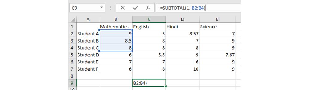
For example, in this dataset, if you want to find the average performance of students A, B and C in mathematics, you can use the SUBTOTAL function as follows: 

=SUBTOTAL(1, B2:B4) 

This will give you the average performance of the three students in the class in mathematics.

8) ROUND Function 

This is a useful function to use when you have data entries in decimals and you wish to round off the numbers to a specific number of decimal points or to whole numbers. 

This function has a simple syntax, beginning with an equal sign, followed by the command- ROUND, followed by a bracket, in which you enter the specific cell value of which you want to round off the decimals, followed by a comma, after which you enter a number, which denotes the number of decimal points you want in your final rounded off value. 

The syntax of this command is =ROUND(cell value, number)

Where number denotes the number of digits or decimal points needed in rounded off value. 

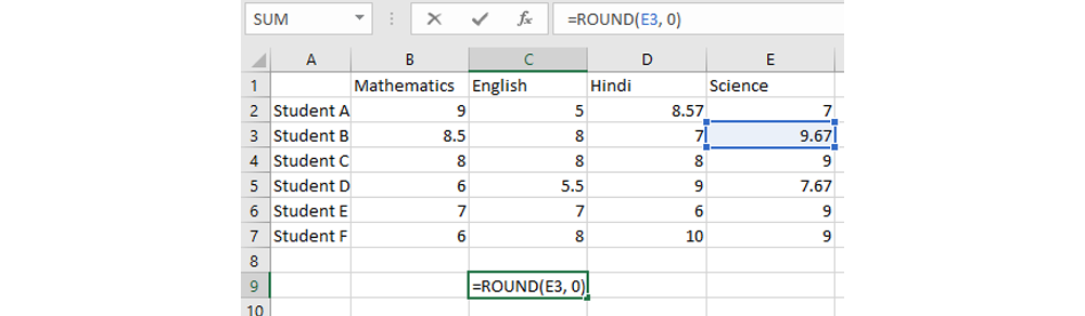
For example in this case, if you want to round off the scores achieved in the science test by student B to whole numbers, you can use the following command: 

=ROUND(E3, 0)

This will give you the score rounded off to the nearest whole number. 

9) MODULUS Function 

The MODULUS function, which is represented as MOD in the Excel function, is a computational command used to find the remainder when a particular dividend is being divided by a divisor. It is a powerful tool to use with a simple syntax, and it is useful when you need to find remaining values after a division has been performed. 

The syntax of the command includes an equal sign (“=”) followed by the main command-MOD, followed by the cell value, which will act as your dividend, followed by a comma after which you enter the number which you want to divide it with (i.e. you divisor). The syntax is closed with the bracket as shown here: 

=MOD(cell value, divisor)

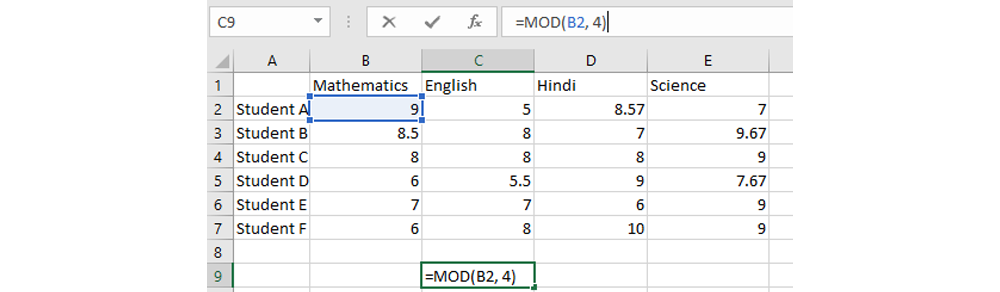
So for example, if you want to divide the cell value in B2 by 4, then the command given will be: 

=MOD(B2, 4) 

This will give you the remainder when 9 is divided by 4, i.e. 1. 

10) POWER Function 

The POWER function is used to calculate a cell value to a particular exponential value. As the command name itself suggests, this command calculates the cell value “to the power of” a certain exponent. 

The syntax of this command includes an equal sign, followed by the main command- POWER, followed by bracket, in which you first enter the referent cell value, followed by a comma, and then the digit which denotes the power to which you wish to raise the cell value. The command is then closed with a bracket. So the final syntax of the command is 

=POWER(cell value, power value) 

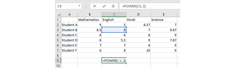
For example, in this dataset, if you wish to calculate the square of the value in cell C3, the command given will be 

=POWER(C3, 2) 

This will calculate the cell value in C3 to the power of 2, i.e. the cell value will get squared.

11) VLOOKUP Function 

The VLOOKUP function, or Vertical Lookup function in MS Excel is primarily used for finding a particular value in a vertical table, with respect to a specific searching value. This feature is extremely useful for quickly looking up values in a large dataset where locating data can be tedious manually. 

The syntax of the VLOOKUP feature involves the following arguments:

• An Equal Sign (“=”)
• The Main Command: VLOOKUP
• Brackets 
• The Column Lookup Value (lookup_value): The Value for which You Want the Corresponding Value  
• The Table Array (table_array): this includes the total table from which you want to fetch the relevant data 
• The Column Index Number (col_index_num): this includes the column number with respect to the table array, e.g. third column or fourth column etc. 
• The Lookup Range [range_lookup]: This indicates whether you want an approximate value for your entry (represented as 1 for TRUE) or the exact value for your entry (represented as 0 for FALSE)

This shall be made further clear with an example:

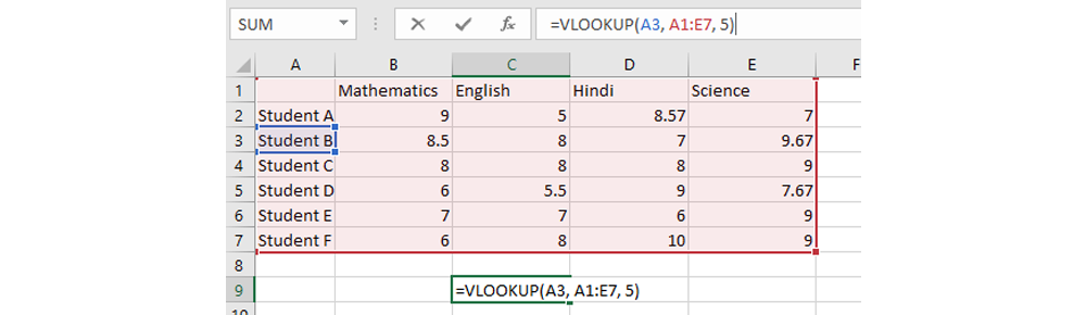
In this dataset, supposing you want to find the test score for student A in the test of science, then you can use the VLOOKUP feature as follows: 

• Type in the item/student for whom you want to find the value (in this case, Student A) 
• To perform the VLOOKUP function enter the following commands: 
  • =VLOOKUP
  • In the brackets, you need to enter the following arguments 
    • (lookup_value): for e.g. Student B
    • (table_array): for e.g. the full table from A1:E7
    • (col_index_num): for e.g. the fifth column which shows the score for science 
  • Following this, you can close the command
  • Press enter and the relevant score value will be displayed in the column. 

12) MINIMUM or MIN Function 

This is a simple searching function in MS Excel in which you use the command to find the lowest or minimum cell value in a range of cells. It stands for MINIMUM and is represented as “MIN” in use. This is useful to use when you have a large dataset and need to quickly find the minimum value from a set of values. 

The syntax includes an equal sign (“=”) followed by the command, i.e. MIN, followed by a bracket in which you enter the cell range and then close the bracket. This will give you the minimum value in your entered data range. The full syntax for the function is 

=MIN(staring cell value:ending cell value)

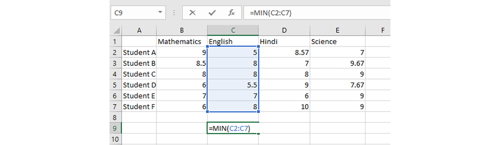
For example, in this given dataset, if you want to find the lowest score achieved in the test of English, you can use the command: 

=MIN(C2:C7) 

13) MAXIMUM or MAX Function

Similar to the MIN function, the MAXIMUM or MAX function is mainly used for finding the highest value in a data range. This is a useful command for a large dataset where it might be manually tedious to locate the highest value. 

The syntax includes an equal sign (“=”), followed by the main command-MAX, followed by a bracket in which the cell range is provided, and then the command is closed with a bracket. The syntax is: 

=MAX(starting cell value:ending cell value) 

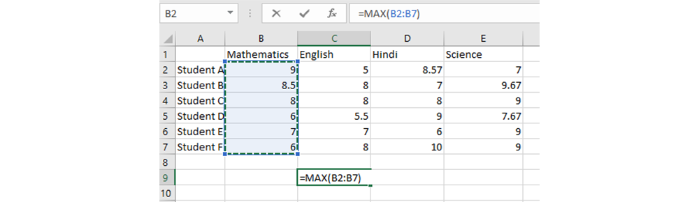
For example, in this dataset if you want to locate the highest score achieved in the mathematics test, you can simply use the command: 

=MAX(B2:B7)

 This command will give you the maximum value in the cell range of B2 to B6. 

14) TODAY Function 

This is a function in Excel which helps you to enter data regarding the current date in a cell. The main use of the TODAY function is to enter the current standard date in a cell from the system. 

The syntax of this command is simply =TODAY()

Note that this command does not require any value within the brackets, since it does not perform a function in reference to a particular cell but fetches system data. 

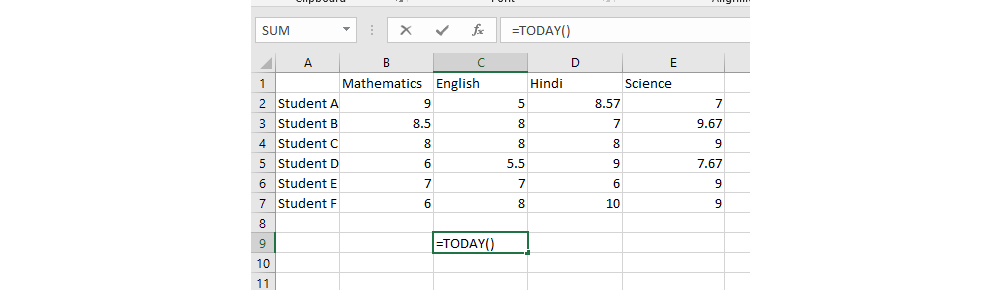
So in this dataset, if you want to enter the date when you performed the operations in the sheet, you can use this function by simply putting the command =TODAY(). 

15) NOW Function 

The NOW function is similar to the TODAY function, the only difference being it fetches system data regarding the date as well as the current time. This feature is useful when you need to record the precise time for data collection/data entry, for e.g. in the case of keeping medical records of blood samples. 

The function has the following syntax: =NOW()

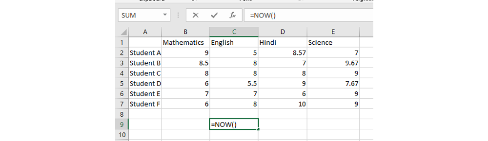
So for instance, in the given dataset, if you want to enter the current date and time, you can simply feed to command and get the data. 

16) LEN Function 

The LEN function in MS Excel is used to calculate the length of the value in a cell, i.e. the number of characters in a cell. The function is useful for calculating the total number of characters in a cell for both textual or string data or numerical data. 

The syntax of the command includes an equal sign (“=”) followed by the main command- LEN, followed by a bracket which encloses the cell values for which the  number of characters is to be calculated, i.e. 

=LEN(cell value)

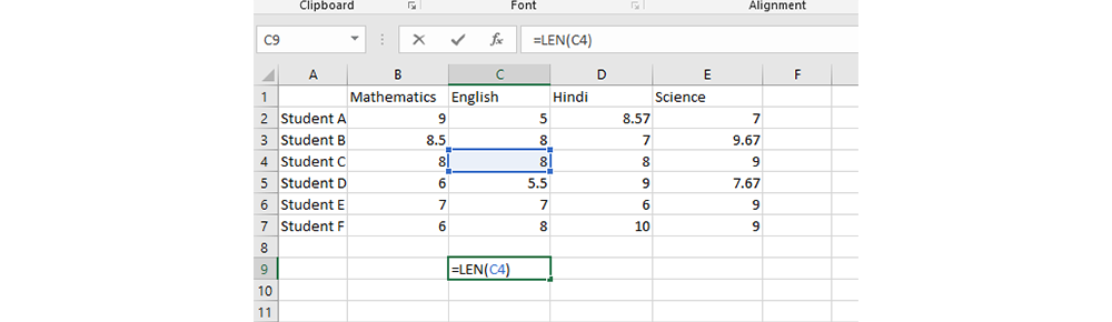
For example, if you want to calculate the number of characters in the given dataset for the cell value C4, you can simply use the command to do so

=LEN(C4)

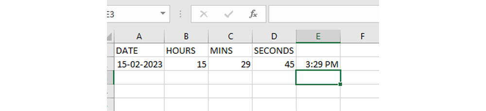
17) TIME Function 

The TIME function is a useful tool when you have data regarding the hours, minutes and seconds recorded in separate cells. The TIME function is used to convert these separate data into a combined time. 

The syntax of the TIME function is a little specific and needs to be kept in mind when you want to convert numerical data into time. The syntax is given here: 

=TIME(Hour, Minute, Second) 

• The meaning of this is that within the bracket, the first cell value (i.e. the first argument) will indicate the hours of the time, and it can range between 0 to 23. 
•  The second cell value (i.e. the second argument) will indicate the minutes in the time, and hence it can have a value between 0 to 59. 
• The third cell value (i.e. the third argument) indicates the seconds and will have a value between 0 to 59.

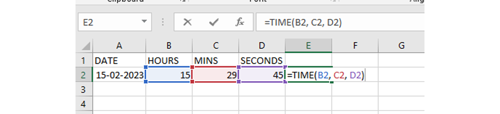
So, if you want to convert the data given in the above data range from B2 to D2, then the command given will be 

=TIME(B2, C2, D2) 

Where 

• B2 represents the Hours
• C2 represents the Minutes and 
• D2 represents the Seconds 

18) REPLACE Function 

The REPLACE function is used to replace a particular part of a text in a cell with content from another cell. This command is useful for replacing texts quickly in a large dataset, but it needs a basic understanding of the arguments in the function before you can use it. The basic syntax of this command is: 

=REPLACE(old_text, start_num, num_chars, new_text) 

Here, 

• Old_text refers to the original cell value in which we want to replace some textual content
• Start_num refers to the position of the character from where you want to start replacing 
• Num_chars refers to the number of characters that you want to replace
• New_text refers to the text that you want to replace the old text with, and it can be a new text or another cell value. 

Consider this example where we want to replace the old text “Student A” with “Student X” here we will use this command: 

=REPLACE(A2, 9, 1, “X”) 

Here,

• The old text is cell A2
• The starting character position is 9 (Note that in this formula the space is also considered a character) 
• The number of characters to be replaced is 1, i.e. just A has to be replaced with X
• The new text is X which is entered within double quotes. 

19) SUBSTITUTE Function 

The SUBSTITUTE function in MS Excel is used to replace a string of text in a cell with a new text when the original text is present more than once within the cell. It has a syntax as follows: 

=SUBSTITUTE(text, old_text, new_text, [instance_num]) 

Where 

• Text refers to the original cell value in which your old text is present
• Old_text refers to the text within this cell that you want to replace, and it is entered within double quotes
• New_text refers to the text that you want instead of the old text 
• [instance_num] refers to the position of the old text that needs to be replaced when it occurs more than once, e.g. second instance or first instance and so on. 

Here is an example: 

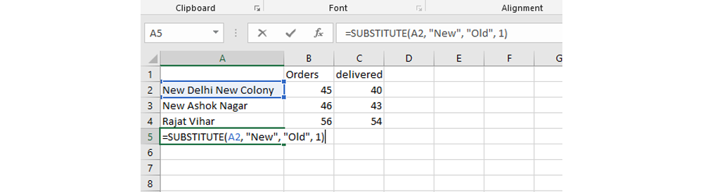
For example you want to substitute New Delhi New Colony entry with Old Delhi New Colony, then in that case you can use the following command: 

=SUBSTITUTE(A2, “New”, “Old”, 1) 

Here the 1 indicates that only the first “New” in the original text is to be substituted with old.

20) TRIM Function 

The TRIM function in MS Excel is used to remove extra spacing in cells to format them into a more concise view. This function is useful to provide a uniform spacing to textual/numerical data which has irregular spacing. 

The syntax simply involves an equal sign (“=”), followed by the main command-TRIM, followed by a bracket within which the cell value is entered and brackets closed: 

=TRIM(cell value)

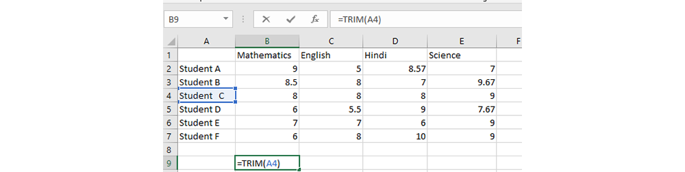
For example, in the given dataset, if you wish to remove the extra spacing between the textual content, to include only single spacing, you can use this command: 

=TRIM(A4) 

In Demand EdTech Tools

Age Calculator Online	BMI Calculator Online
Fraction Calculator Online	EMI Calculator Online
Gallon to Liter Calculator Online	ROI Calculator Online
INR to USD Converter Online	Meter to Feet Converter Online
Percentage Calculator Online	University Eligibility Tool

Conclusion 

There are a number of useful and quick to use formulae and functions in MS Excel that can become handy when you are handling large databases and datasets. Over time, when you use these functions frequently, you will get accustomed to using them in practice. The interface of Excel for using the functions is also very helpful as it provides you with the arguments as a prompt, which can help you feed data to run the command accordingly.